|
SIMPLICITY:
CAS Geometry
Distances
Equidistances
Constant Distances
Algebraic Eqs. and
Inequations
Angles
Taxicab Distance
Fields
VERSATILITY
List of Polylines
FLEXIBILITY: Elastic geometry
Elastic Geometry
Newton's Principia
Tensegrities |
Abstract
Since its inception, GeoGebra has
been
specifically designed to display the dual representation, both
graphical and
algebraic, of mathematical objects. In this presentation, as the central
focus,
I will show some procedures that exploit the didactic possibilities of this
duality.
These procedures, presented to students aged 15 or 16, are so simple,
engaging and quick to create that they allow the students themselves to
generate and use them from scratch... with great success!
Despite their simplicity, we will see that they are so powerful that they
enable us to delve into mathematical depths that are practically
unapproachable in the high school classroom without the assistance of GeoGebra,
ranging from algebraic structures (such as fields) to non-Euclidean metrics (like
the taxicab metric). |
Note: All the GeoGebra constructions linked on this webpage
have been created
by the presenter of this content. None
of them, except for the
Bubbles construction,
make use of JavaScript programming.
The Author
In my 40 years of teaching as
a High School Teacher, in the pursuit of fostering the interest of students,
I have researched the relationship between Mathematics and other areas as
diverse as Games
 ,
Perception
,
and Music
.
The advent of Dynamic Geometry brought new and significant opportunities to
engage students and promote the creation of their own constructions. ,
Perception
,
and Music
.
The advent of Dynamic Geometry brought new and significant opportunities to
engage students and promote the creation of their own constructions.
My relationship with GeoGebra dates back to 2005 when I first encountered
this program created by Markus Hohenwarter [7],
although I had already worked with other dynamic geometry software. Two
years later, in 2007, Professor Tomás Recio
invited me to the International Center for Mathematical Meetings (CIEM
, Cantabria)
which brought together several Spanish high school teachers who were
pioneers in the educational use of dynamic geometry. During that
meeting, I defended the efficiency of GeoGebra [10] compared to other
software like
Cabri. One outcome of that gathering was
the formation of the G⁴D
group,
consisting of J.M. Arranz , J.A. Mora , M. Sada and
the author of this text
.
Two years later, from the Ministry of Education of Spain, Antonio Pérez ,
who was then the director of the Institute of Educational Technologies (ITE,
now INTEF ),
entrusted me with the task of conducting courses for training Primary and
Secondary Education teachers in GeoGebra [11,
13].
Additionally, I was tasked with creating a set of complete activities
(including topic introductions, constructions to explore, and
questionnaires) for students, categorized by subjects and levels, which we
named
the Gauss Project [14,
1]. Simultaneously, Tomás
launched the first Spanish-language GeoGebra Institute, the GeoGebra
Institute of Cantabria ,
of which I have been a Trainer since its inception.
Introduction
The main objective of this conference is to demonstrate the close relationship between
algebraic and geometric procedures using GeoGebra. A significant portion of the time will
be dedicated to presenting activities that can be approached by secondary
education
students through constructions carried out by themselves. Beyond sporadic use
for exploring specific content, this type of
construction gains its full didactic power in mathematics education based
on competence acquisition.
In the first part of this presentation I will detail very simple
procedures that harness the strong interconnection between
geometry and algebra that gives its name to GeoGebra (hence the title
of Principia) and enable secondary school students (around 15
or 16 years old) engage in mathematical explorations that are "in principle"
beyond their reach, leaving the heavy algebraic and geometric calculations
to the powerful tools of GeoGebra, much like we currently rely on
calculators and spreadsheets for tedious arithmetic calculations.
In particular, the ease with which we can create parallel lines and
circles will aid us in constructing a dynamic offset whose
colorful trace allows us to visualize a wide variety of geometric loci.
Simultaneously, the Computer Algebra System (CAS), applied to
Euclidean distances, will facilitate the creation of implicit curves that
conform to these loci. We will also see how to
occasionally convert these implicit curves into algebraic equations and
inequations.
We will expand the use of CAS to angles and also address other
non-Euclidean distances, such as the taxicab distance.
We will conclude this first part with a reciprocal example, wherein
resorting to geometry will aid us in visualizing and manipulating the
concepts and properties inherent to the algebraic structure of a
field.
In the second part, I will showcase some ideas for creating slightly more
sophisticated yet equally captivating constructions, which can serve as
models to be analyzed or modified by students.
Firstly, we will explore how GeoGebra's lists facilitate the
incorporation of a substantial amount of information. As an example, we
will represent the coastlines of continents in a single list, creating a
template of the Earth.
Next, we will employ vectors to instantaneously modify (thanks to the
GeoGebra scripts) the position of points according to our
interests. These vectors can be used to combine repulsive forces (like
particles of the same charge), attractive forces (similar to those used by
Newton to formulate his universal law of gravitation), or simply reactive
forces (as in elastic collisions).
Furthermore, we can use vectors to create an "elastic geometry".
In this context, points do not possess a fixed location, but rather their
position at each moment is the result of the application of the
aforementioned forces. For instance, in elastic geometry, a point is not "on" a circle, but is
inevitably drawn towards it, it has "its limit" in it.
Lastly, as an application of this type of elastic
geometry, we will examine examples of tensegrities constructions.
SIMPLICITY:
CAS Geometry
GeoGebra: Geometry and Algebra
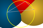
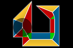
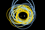
Since its inception, GeoGebra has enabled the rapid and straightforward
construction of geometric models, enhancing learning, teaching, and
research. This ease of use contributes to the IKEA effect
(we value more what we are capable of building ourselves, hence the
success of classic construction games, such as
Meccano or Lego). Here, I present one of the constructions that
I showcased at the 2007 CIEM meeting [9], where I
advocated for the use of this program in education. I have
chosen this one because Markus popularized it by featuring it for years at
the header of the official GeoGebra website
.
Since then, GeoGebra has seen significant development. We can create
countless models and applications related to areas such as Arithmetic,
Equations, Functions, Isometries, Complex Variables, Statistics,
Probability...
The variety of procedures is also immense: from slicing a hypercube into
sections [15]
to automatically proving a proposition [12,
17, 18, 28].
It is evident that what characterizes dynamic geometry is precisely
its dynamism. Just like in most animals with a visual system, evolution
has triggered a mental alert when any object or entity in our surroundings
starts moving. Therefore, motion is a natural and excellent means to focus
attention.
However, how can we easily visualize geometric loci without resorting to complex constructions or
using cumbersome algebraic
equations? We will see that one possible answer is to use the CAS.
Distances
The mathematical concept I will revolve around is a fundamental one: distance.
|
When placing
a point in a space, the concept of distance to it behaves like what
physicists call a "field": it doesn't manifest until we introduce
another object into it.
We will employ two simple procedures to visualize geometric places
related to distance: the creation of implicit curves and the use
of dynamic offset with activated trace. |
Classic Method:
Sequences of Parallel
Curves
(Static Offset)
Using the UnitPerpendicularVector command (and its
opposite vector), it's simple to create sequences of parallels to a line
at progressive distances. For each line r, we find a pair of
sequences:
Sequence(Translate(r, k
UnitPerpendicularVector(r)), k, 0, 20, 0.2)
Sequence(Translate(r, -k
UnitPerpendicularVector(r)), k, 0, 20, 0.2)
Thanks to the CurvatureVector command and the
Locus tool, we can generalize parallelism to many curves (offset ).
If P is a point on curve c, the two parallel
curves at distance k will be given by the locus of the points:
P ± k
UnitVector(CurvatureVector(P, c))
Note that, in general, offset curves are not congruent with the
original curve. In other words, parallel curves are not
simple translations, except in the case of lines.
However, in the case of the circle (let's assume with
center O and radius 4), whose offset is also a circle, we
don't need the CurvatureVector command or the Locus tool,
as it's sufficient to vary the radius of the original circle appropriately:
Sequence(Circle(O, 4 + k), k, 0, 20,
0.2)
Sequence(Circle(O, 4 – k), k, 0, 20,
0.2)
Furthermore, if we consider a point O as a circle
with radius 0, we obtain a unique sequence of offsets centered on it:
Sequence(Circle(O, k), k, 0, 20,
0.2)
|
In summary, we can easily create sequences of parallels to lines,
circles and points. |
Dynamic Offset with
Activated Trace
Now we will replace each sequence of parallels with a single dynamic
parallel. As before, using the UnitPerpendicularVector
command (and its opposite vector), it's straightforward to create parallels
to a line at a given distance d.
For each line r, we find a pair of parallels:
Translate(r, d
UnitPerpendicularVector(r))
Translate(r, –d UnitPerpendicularVector(r))
Thanks to the CurvatureVector command and the
Locus tool, we can generalize parallelism to many curves (offset).
If P is a point on curve c, the two parallel curves at
distance d will be given by the locus of the points:
P ± d UnitVector(CurvatureVector(P, c))
Note that, in general, offset curves are not congruent
with the original curve. In other words, parallel curves are not simple
translations, except in the case of lines.
However, in the case of the circle (let's assume with
center O and radius 4), whose offset is also a circle, we
don't need the CurvatureVector command or the Locus tool,
as it's sufficient to vary the radius of the original circle appropriately:
Circle(O, 4 + d)
Circle(O, 4 – d)
Furthermore, if we consider a point O as a circle
with radius 0, we obtain a unique sequence of offset centered on it:
Circle(O, d)
|
In summary, we can easily create sequences of offsets of lines,
circles and points. |
Also, we can create the intersection points of two objects
and the corresponding locus. The problem with using the Locus
command or tool is that in many situations (more complex than the one
shown here) it's not possible to use it properly.
Since GeoGebra is a Dynamic Geometry program, we can not only move
geometric objects at our will but also establish automatic animations [22].
To achieve this, we add a trace to the offset and choose a
decreasing value of d (opposite to a slider "increasing once").
Note: alternatively, we can choose an increasing value for d (increasing
once) and assign it a speed of -1 instead of 1.
By doing so, simultaneously offsetting a point and a line, for instance,
we can visualize the parabola through color contrast.
|
The advantage
of using offset over implicit curves, which we will see next, is that it
allows us to pause the procedure's playback at any time and observe how
the traces of the lines intersect. This helps us understand why these
intersection points are part of the sought-after locus. |
Implicit Curves
from Definitions in CAS
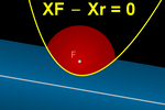
A parabola can be defined as the locus of points in the plane equidistant from a line (directrix) and
an external point (focus).
Locating one point (the vertex) is easy, but how do we locate the others?
With GeoGebra, we can create a free point to explore the situation and mark
those positions where both distances are equal. It's quite instructive
but, after several exercises, it becomes tedious.
Alternatively, we can construct a generic point that defines the locus,
but this construction will only work for this case or similar cases.
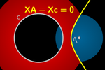
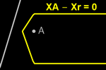
We can also create the implicit curve by defining
an arbitrary point X(x,y) in the CAS View:
X:= (x, y)
the distance from X to the
focus F:
XF(x,y):= Distance(X, F)
the distance from X to the directrix r:
Xr(x,y):= Distance(X, r)
and by equating both distances:
XF – Xr = 0
GeoGebra uses numerical algorithms to create this implicit curve, so small
errors or omissions may appear in some cases.
Note: At least for now,
GeoGebra does not represent equations of this type in three variables.
That is, it recognizes x² + y² + z² = 16 as a sphere, but it does not
recognize the equivalent equation (sqrt(x² + y² + z²))² = 16 as such.
Equidistances
Now we just have to use those simple tools to investigate a wide variety
of situations with their assistance.
From now on, we consider the distances from an arbitrary point X(x,y)
to A and B
defined as:
XA(x,y):= Distance(X, A)
XB(x,y):= Distance(X, B)
to a line r as:
Xr(x,y):= Distance(X, r)
and to a circle c as:
Xc(x,y):= Distance(X, c)
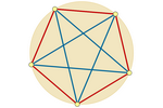
Equidistance to Two or Three Points
By contracting the circles with the activated trace, at each point in the
plane, the color of the nearest center remains, resulting in the
perpendicular bisector.
The implicit curve of the perpendicular bisector of AB is given by the
equation:
XA – XB = 0
In the case of three points, we can visualize the circumcenter [2]
of the triangle they form.
|
We have already seen.... |
Equidistance to a Point and a Line
By simultaneously moving a
parallel line to the line r and to the circle centered at A, with the
trace activated, the color of the nearest object (line or point) remains
at each point. This gives us the corresponding parabola. As we have
already seen, in this case, it's also easy to construct this
locus.
|
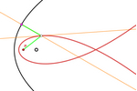
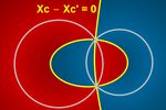
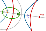
Equidistance to
a Point and a Circle
If the point is inside the circle, we obtain an ellipse, and if it's
outside, a branch of a hyperbola.
The implicit curve of the ellipse or branch of the hyperbola is given by the
equation:
XA – Xc = 0
Note that a construction similar to the one for the parabola also allows
us to generate this locus.
|
Furthermore... |
Equidistance to
a Point and a Conic
These constructions for the loci of points
equidistant from a point and a conic are very similar to the construction
for points equidistant from a point and a circle. However, the
equation is much more complicated to find.
|
Equidistance to
Two Lines
By simultaneously moving parallels to two lines, with the trace activated,
the color of the nearest line remains at each point, yielding the angle
bisectors. In the case of three lines, we can visualize the incenter and
the excenters of the triangle they determine.
As a specific case, we can visualize the medial axis
of
a polygon as the boundary (composed of segments and arcs of parabolas) between
the surviving traces.
Similar to before, we can also easily visualize and construct the
corresponding geometric locus of the angle bisector.
Equidistance
Line-Circle and Two Circles
The locus of points equidistant from a line and a circle is generally
composed of one parabola or, if they intersect, two parabolas.
The locus of points equidistant from two circles is generally composed of a
branch of a hyperbola or, if they intersect, an ellipse.
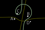
Voronoi Diagram
and Similar Maps

Although the implicit curve is faster to create and use,
the offset method allows us to tackle problems that the implicit curve
cannot address. For instance, if instead of applying the offset method to the
equidistance between two points (the bisector), we apply it to several
points, we obtain the Voronoi diagram (or Thiessen polygons).
Similarly, we can also create the map of regions closest to a
collection of lines or circles.
Note: GeoGebra's Voronoi command does not color each
region. A dynamic way of achieving this can be seen here
.
Equidistance to
Two Curves
We can apply the offset method to two curves as long as we can calculate
the normal vector at each point of both.
In situations where calculating the normal vectors isn't feasible, we can always
generate a heat map using the dynamic color scanner technique [3,
19, 26, 27,
31].
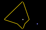
Constant Distances
Point-Point
When the sum of the distances from the points of the sought-after
locus to points A and B is constant, we obtain an ellipse.
When the difference of the distances from the points of the
sought-after locus to points A and B is constant, we obtain
a branch of a hyperbola. (In the case where the constant is 0, we obtain
the perpendicular bisector.)
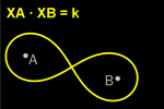
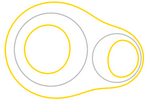
When the product of the distances from the points of the
sought-after locus to points A and B is constant, we obtain
a Cassini oval
.
If the constant coincides with the square of half the distance AB, we
obtain a Bernoulli lemniscate
.
Surprisingly
,
when the quotient of the distances from the points of the
sought-after
locus to points A and B is constant, we obtain
a circle. (In the case where the constant is 1, we obtain the perpendicular
bisector.)
Constant Ratio Point-Line
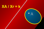
When the quotient of the distances of the points of the sought-after locus to
point A and line r is a constant k, we obtain a
conic section, which will be an ellipse, parabola or hyperbola depending on
whether the value of k (eccentricity) is less than 1, equal to 1,
or greater than 1, respectively
.
Constant Linear
Combination
We can generalize the sums and differences to any linear combination of
distances between points, point and line, point and circle,
etc.
This leads to conic sections and quartic curves (Cartesian ovals, products
of lines...), Pascal's limaçon
,
as well as higher-degree curves formed as products of the aforementioned
curves.
|
Furthermore... |
Constant
Logarithmic Linear Combination
 We
can also generalize products and quotients to any linear combination
of logarithms of distances. The degree of these curves
depends on the chosen value of q. We
can also generalize products and quotients to any linear combination
of logarithms of distances. The degree of these curves
depends on the chosen value of q.
|
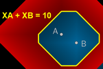
Constant Sum to
Three or Four Points
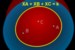
In the case of a constant sum k of distances to three points A,
B and C, you simply need to input:
XA + XB + XC = k
To perform the
offset, what we do is overlay the trace of ellipses Ellipse(A, B,
(k–h)/2) with circles Circle(C, h), where h is a positive real
parameter that decreases from the value of k to zero. The boundary points
of color will then be precisely the points that satisfy:
Ellipse(A, B, (k–h)/2) = Circle(C, h)
which is
equivalent to the sum of the distances from those points to A, B
and C being exactly the predetermined quantity k (since XA + XB = k
– h, XC = h). This way, we can display a 3-ellipse
.
In the case of four points the traces of two ellipses overlap, determining a
4-ellipse.
Note: An
algebraic approach to this situation, also using GeoGebra, can be seen in
this article [8] by Zoltán Kovács.
Algebraic
Eqs. and
Inequations
Equidistance to
a Point and a Circle: Algebraic Equation
Previously, we directly defined the distance from a
point X(x,y) to the circle c as:
Xc(x,y):= Distance(X, c)
With this, the equation for the points equidistant from a point A and a circle
reduces to:
XA – Xc = 0
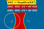
If the circle has a center O and radius s, we can redefine the
equation as:
|XO – s| = XA
This redefinition allows us to visualize the two branches of the
hyperbola. To achieve this, we transform the previous irrational
equation into an algebraic equation by squaring it to eliminate the roots
(reaching the following expression is straightforward, as it doesn't require
grouping, simplification or cancellation steps, but it's also okay to
assist students with limited algebraic resources in solving this small
exercise—the result is worthwhile):
(XA² – XO² – s²)² = 4s² XO²
Moreover, algebraic equations have the advantage of enabling
representation of the corresponding inequations without resorting to the
offset method. For this, we simply define:
XA2(x,y) := Simplify(XA^2)
XO2(x,y) := Simplify(XO^2)
This way, we can introduce the inequations:
(XA2 – XO2 – s²)² < 4s² XO2
(XA2– XO2 – s²)² > 4s² XO2
Constraints on Inequation Representation
However, not always does the algebraic equation allow GeoGebra to
represent the corresponding inequations. As shown in the official manual
,
this representation is limited to the following cases:
-
Polynomial inequalities in one variable, like x³ > x + 1
-
Quadratic inequalities in two variables, like x² + y² + x y < 4
-
Linear inequalities in one of the variables, like 2x > sin(y) or y < sqrt(x).
When we find the algebraic equation corresponding to XA – XB = k, we obtain
the same as the one corresponding to XA + XB = k:
4 XB2 XA2 = (k² – XA2 – XB2)²
This equation reduces to a quadratic in two variables, allowing
GeoGebra to represent its corresponding inequations.
Note: The common quadratic equation of
the ellipse and hyperbola is nothing but the general equation of
a conic:
a x² + b x
y + c y² + d x + e y + f = 0
where the ellipse and the hyperbola differ only by the sign of the discriminant b² – 4 a c.
However, the algebraic equation corresponding to XA XB = k doesn't represent a
conic, so GeoGebra can't represent the corresponding inequations.
On the other hand, the algebraic equation corresponding to XA = k XB becomes a
conic once
again, allowing GeoGebra to represent the corresponding inequations.
Equal Sums of
Distances to Two Pairs of Points
If we input XA + XB = XC, the resulting locus corresponds to the
intersection of a family of ellipses XA + XB = k, and a family of circles XC =
k, as the parameter k varies.
In the case of four points, XA + XB = XC + XD corresponds to the
intersection of two families of ellipses.
Note: Calculating the minimum and maximum
values of k that ensure intersection is not straightforward. An approach
can be seen in [6].
The case XA + XB = Xr is also presented, along with the representation of
the corresponding algebraic equations.
Families of Curves
In conclusion, the field to explore can expand indefinitely. As final
examples with distances, let's observe some results involving powers.
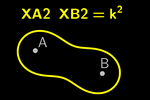
It is easy to demonstrate that the representation of XA2 + XB2 = k, with k
constant, is a circle centered at the midpoint of A and B.
Note: The radius of that circle is sqrt(k/2 − (x(A-B)/2)²
− (y(A-B)/2)²).
From this, we deduce that the locus where the sum of the squares of
distances to several points is constant is a circle centered at the
midpoint of those points.
Furthermore, taking D = XA2, we can observe that the real-plane
representation of any polynomial p(D) is exclusively composed of
one or more circles.
Note: This follows from the Fundamental
Theorem of Algebra, since p(D) can be decomposed by factors (D − c), where
c is a complex number. If c is non-negative real, then D − c = 0
corresponds to a circle with radius the square root of c. Otherwise, nothing is
displayed.
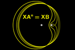
Here, we also see that we can represent multiple curves of the same family,
such as XAn = XB and observe
their behavior simultaneously.
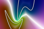
Angles
The following is one of the images generated using the dynamic color
scanner that I particularly like. The scanner has tremendous versatility, it
can create a heat map for virtually any situation
[3,
19, 26, 27,
31].
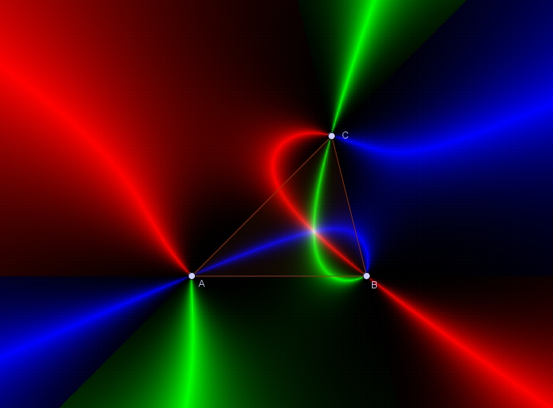
In this case, the first isogonic point I1 is visualized by
intersecting the loci that see each pair of sides of the triangle under
the same angle.
Note: I1 coincides with the Fermat point
when the triangle's largest angle is not greater than 120 degrees; otherwise,
the Fermat point coincides with the vertex corresponding to that angle. It
can be calculated directly as the triangle's center X(13)
:
I1 = TriangleCenter(O, A, B, 13).
However, constructing the scanner takes some effort. But we can use CAS to
define not only distances but also angles. If someone still thinks that
using the expression
XA instead of sqrt((x − x(A))² + (y − y(A))²)
doesn't save much work, perhaps they'll reconsider now when they can use
the expression OXA, defined in the CAS view as:
OXA(x,y):= Angle(O, X, A)
instead of its algebraic equivalent (with O=(a,b) and A=(c,d)):
cos–1((a c – a x + b d – b y – c
x – d y + x² + y²) sqrt(a² c² – 2a² c x + a² d² – 2a² d y + a² x² + a² y²
– 2a c² x + 4a c x² – 2a d² x + 4a d x y – 2a x³ – 2a x y² + b² c² – 2b² c
x + b² d² – 2b² d y + b² x² + b² y² – 2b c² y + 4b c x y – 2b d² y + 4b d
y² – 2b x² y – 2b y³ + c² x² + c² y² – 2c x³ – 2c x y² + d² x² + d² y² –
2d x² y – 2d y³ + x⁴ + 2x² y² + y⁴) / (a² c² – 2a² c x + a² d²
– 2a² d y + a² x² + a² y² – 2a c² x + 4a c x² – 2a d² x + 4a d x y – 2a x³
– 2a x y² +
b² c² – 2b² c x + b² d² – 2b² d y + b² x² + b² y² – 2b c² y + 4b c x y –
2b d² y + 4b d y² – 2b x² y – 2b y³ + c² x² + c² y² – 2c x³ – 2c x y² + d²
x² + d² y² – 2d x² y – 2d y³ + x⁴ + 2x² y² + y⁴))
Naturally, this expression is merely a development deduced from the
dot product of two vectors:
vO(x,y):= Vector(X, O)
vA(x,y):= Vector(X, A)
OXA(x,y):= acos((vO vA)/(|vO|*|vA|))
The significant advantage, besides convenience, is that the Angle command allows us
to explore angular relationships without needing to know even the basic
operations with vectors, like the dot product.
Here, we can see, for example, the locus corresponding to points that form
an angle (in radians) equal to the distance to point A with segment OA:
OXA − XA = 0
Note: Circles whose arcs span an angle OXA equivalent to XA radians have centers:
(O + A)/2 ± PerpendicularVector(OA)/(2 tan(XA))
And those that see segments OA and OB from the same angle:
OXA − OXB = 0
Finally, the intersection of this latter locus with the one corresponding to the
equation OXA – AXB = 0 is the sought-after Fermat point.
Taxicab Distance
Note: This section arose due to the lockdown declared in
Spain in 2020 as a result of the COVID-19 pandemic. The Education Department of
Asturias, the region where I worked as a teacher, decided to replace
in-person classes with online ones and also decreed the obligation not to
advance curricular material in any subject. This led me to look for a field of
mathematical exploration beyond the official curriculum but within the reach of
10th-grade students (around 15 or 16 years old). For the students, it was
exciting to know that they were investigating a topic virtually unknown to the
vast majority of math teachers. Additionally, the change in metric brought about
a lot of surprises and questions. A mathematical celebration.
Let's now step out of the familiar Euclidean metric:
|
The taxicab
distance (also known as Manhattan distance) is especially simple to
introduce as a research project in secondary education, as its algebraic
form reduces to linear equations. |
Minkowski Distances
The shape of the circle is significant in any plane geometry. Here, we see the
definition of the Minkowski distance
from an arbitrary point X(x, y)
to the origin O.
XO(x,y):= (|x|p+|y|p)1/p
For p=2, we have the Euclidean distance. For p=1, we have the taxicab
distance. By varying p, we can observe how the shape of the circle evolves in each
case.
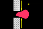
Taxicab
Geometry
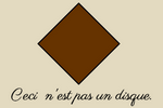
Indeed, as Magritte would say, Ceci n'est pas un disque
(This is not a disk)
,
but we will see that it can indeed be the representation
of a circle if we consider the Taxicab metric.
I will use the prefixes T and E to distinguish between the Taxicab metric
and the Euclidean metric.
Note: Despite the fact that a T-circle has a square
shape, Magritte would probably still assert -rightly- that the T-circle we
see is only a representation, an image of the disk. However, furthermore,
here, unlike what happens with a pipe, the represented disk is a mental
abstraction (an ideal mathematical form) instead of something material,
which makes the potential confusion even greater.
In Taxicab metric (or Manhattan
metric), distances are measured horizontally and vertically,
never diagonally. Thus, the T-distance from
an arbitrary point (x, y) to point O is the sum of the
horizontal and vertical differences, in absolute value, of its coordinates:
XO(x,y) := |x – x(O)| + |y – y(O)|
|
Unlike in Euclidean metric, GeoGebra does not have the
T-distance command implemented, so we will have to formulate both the
distance between two points and the distance between a point and a line
"manually", providing both formulas to the
students. |
Just as GeoGebra renders a segment by fitting it into the pixel grid of the
screen, we can imagine a diagonal segment composed of horizontal or
vertical segments as small as we want: the T-distance between two points B and C
will not change.
The T-distance between B and C will also be the same for any increasing or
decreasing arc of a function whose graph goes from B to C.
|
In taxicab
geometry, there can be infinitely many minimal paths between two
different points. |
All of this does not simplify geometry but complicates it. This is
because the length of each segment is not uniform in direction but
depends on its slope.
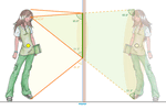
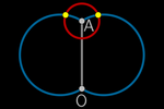
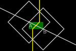
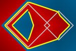
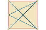
In the E-illusion shown [21],
the blue square appears to change size, but it's only a perception
problem that disappears when you see its sides completely (click on the blue
square). Explanation: when the corners are visible, we estimate the size
of the square by its diagonal; when they are not, we value it by the
distance between opposite sides (side length).
However, in taxicab geometry, the blue square actually varies its area
based on the slope of its sides (while both the T-length of its sides
and its angles remain constant).
Analyzing the square in detail, we see that the T-perimeter of the blue
square and the yellow square is the same, but the area is not: the area
of the yellow square is (b + c)², but the area of the blue square is b² +
c², which is minimal when b = c. Therefore, in taxicab
geometry, the T-areas coincide with the E-areas, but:
|
The area of a
T-square is NOT, in general, equal to the square of its side. |
We can imagine the T-circle as a compression of the E-circle. Due to the
non-uniform T-length in each direction, the T-circle compresses into
a square shape, with its diagonals parallel to the Cartesian axes.
Basic T-Constructions
If we fix a point O in the plane, we can consider the taxicab distance
from the rest of the points to O.
As we have seen, the points that are T-equidistant from O form a square
(with diagonals parallel to the axes). If the radius is r, the perimeter
is 8r, so the ratio between the T-circumference and its T-diameter is 4
(instead of 𝜋).
By fixing another point I different from O, we establish an orientation
O→I and a line. We will take the T-distance from O to I as the unit. We can
continue to think of the T-lines as if they were E-lines, as only the way
of measuring each segment changes. Remember that pixels force GeoGebra to
draw lines composed of horizontal and vertical segments!
Given a point A on the line r, there exists only another point A' on this line
at the same distance from O as A. This T-symmetric coincides with the
E-symmetric point.
For two distinct points A and B, we can find all the points equidistant
from them.
This T-perpendicular bisector does not coincide with
the Euclidean perpendicular bisector.
By intersecting the T-perpendicular bisector with the line, we obtain the
midpoint, which coincides with the Euclidean midpoint.
Perpendicular and parallel lines are the same as in Euclidean
geometry, but the orthogonal projection of a point onto a line does not
generally provide the nearest point on the line. (Moreover, "nearest point"
is not uniquely determined when the line has a slope of 1 or –1.)
To perform a T-inversion
,
we move points A and I to the horizontal line passing through O, invert
(x(A), y(O)) on the dashed E-circle with center O passing through (x(I), y(O)), and create similar triangles that guarantee the new inversion.
The T-inverse of A does not coincide with the
E-inverse of A.
T-Angles
In the unit T-circle, we can define the T-radian exactly the same way we
define an E-radian in the unit E-circle. To T-measure an angle, it's
sufficient to measure the T-length of the corresponding (straight) arc on
the unit T-circle. A T-circle has 8 T-radians.
Perpendicularity and parallelism are preserved under rotations, but, in
general, T-distances are not invariant with respect
to E-rotations... nor with respect to T-rotations! In fact, one of the
peculiarities of T-distance is that it is sensitive to the orientation of
lines: a segment, when T-rotated, no longer measures the same.

Cartoon of Mafalda, by Quino
"It's quite a puzzle, isn't it?
How on earth
does time manage to round the corners on square clocks?"
The sum of the angles in any T-triangle is 4 T-radians. A T-triangle can
be equilateral or equiangular, but it can never be regular.
Any E-square is also a T-square. But because the taxicab distance is not
uniform in every direction, these two T-squares have the same perimeter
(though not the same area):

The square on the left is also a T-circle.
The one on the right is not.
Trigonometric T-functions are much simpler than their Euclidean
counterparts. For example, the T-sine function is not only
non-transcendent but also piecewise linear. The T-tangent function is
composed by piecewise E-hyperbolas.
Note: One possible expression for the T-sine function
is: tsin(x) = 1 – 2 |1/2 - x/4 + 2 floor(1/4 + x/8)|. Thus, the
T-cosine function can be defined as tcos(x) = tsin(x+2). The T-tangent
function is a piecewise homographic function
.
T -Equidistances
When contracting T-circles with the trace activated, at each point in
the plane the color corresponding to the nearest center survives.
With multiple points, we can visualize the Voronoi diagram and compare it
with the one corresponding to the Euclidean distance.
To analyze the equidistance point-line, we need to determine the distance from
a point (x, y) to a line r: a x + b y + c = 0. This distance is (this
formula is provided to students and can be directly introduced in the
algebraic view):
Xr(x,y) = |a x + b y + c| / Max(|a|, |b|)
From the point-line equidistance the T-parabola arises, while from the
point-circle equidistance the T-ellipse and the T-hyperbola emerge.
If we consider equidistance to the sides of a polygon, its skeleton
and median axis arise. We can traverse it with a bitangent disk to
verify this.
Finally, we can also find the T-equidistant path between two curves,
either through offset (as shown here) or by generating a heat map.
T-Conics
As we have seen before, the T-circle takes on a square shape (with diagonals parallel to the axes).
The T-ellipse generally has the shape of an octagon. If points A and B lie on the
same vertical or horizontal line, it takes on a hexagonal shape. When the
constant sum coincides with the T-distance from A to B, the ellipse
degenerates into a rectangle with diagonal AB.
The T-parabola is generally formed by two rays (either horizontal or
vertical) and two segments.
Finally, each branch of the T-hyperbola is generally formed by two rays
(either horizontal or vertical) and one segment.
|
Furthermore... |
T-Constant Linear
Combination
Just as we did in Euclidean geometry, we can
generalize the constant sum or difference to any linear combination.
T-Constant Logarithmic Linear
Combination
It's worth noting that distances inversely
proportional to two points do NOT give rise to T-circles, as was the case
with Euclidean metric.
This implies that the possible definition of a circle as tbe locus of points
in the plane whose ratio of distances to two fixed points is constant is
not valid for every metric.
|
T-Sphere
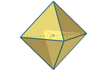
A T-sphere is formed by the points in space that are T-equidistant from
its center. It takes on the shape of a regular E-octahedron (which is not
T-regular, as T-regular triangles do not exist) with its diagonals
parallel to the axes. It can also be generated by T-rotating a T-circle
around the
horizontal or vertical diameter.
|
The loci that appear in taxicab geometry invite us to ask: what does
"something" need to have in order to be that "something"? What characterizes an
object? For instance, is the E-sphere round because its points are
equidistant from its center, or is it round due to the uniformity in the
direction that Euclidean distance possesses? |
T-Ellipsoid
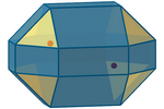
A T-ellipsoid is the locus of points in space whose sum of T-distances to
the foci is constant (k). It generally takes on the shape of a polyhedron
with 18 rectangular faces and 8 triangular faces (which are E-regular but
not T-regular).
The T-ellipsoid degenerates into an E-cuboctahedron when the absolute
differences of the coordinates of the foci coincide; it degenerates into
an
E-cube when these differences also coincide with k; and it degenerates into a
T-sphere (regular E-octahedron) when the foci coincide.
For certain special positions of the foci, a T-ellipsoid appears with all
its faces formed by regular E-polygons, but it is neither a regular or semiregular
E-polyhedron,
as its vertices are not uniform.
Finally, when the T-distance between the foci is equal to k, we obtain an
orthoedron.
Fields
Let's return to our familiar Euclidean metric. So far, we have used algebra
to facilitate the observation of loci. Let's now see an example
of the reciprocal process: using geometry to facilitate the observation of
algebraic structures.
Normally, we think of algebraic structures (groups, rings, fields...) as
something inherent to certain numerical structures, like integers or
real numbers.
However, we can easily create equivalent geometric structures, with the
advantage that we can visualize each arithmetic operation as a
geometric construction.
Prelimin ary
Constructions
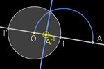
If we fix a point O in the plane, we can consider the (Euclidean)
distance from the rest of the points to O. We will denote OP as the
distance from O to P.
The points equidistant from O form a CIRCLE.
By fixing another point I different from O, we establish a DIRECTION, an
ORIENTATION O→I and a LINE r.
We will take the distance OI as the UNIT. Additionally, two points on the line limit a
semicircle. A point P is on the line r if it satisfies any of these
equalities:
OI = OP + PI (P is between O and I)
OP = OI + IP (I is between O and P)
PI = PO + OI (O is between P and I)
-
Point reflection (symmetry): If A is on the line, there exists only
another point A' on it at the
same distance from O as A.
Perpendicular bisector: Given two distinct points A and B, we can find all
the points that are equidistant from them.
Midpoint: Intersecting the perpendicular bisector with the line r, we
obtain the midpoint MAB.
Perpendicular: The perpendicular bisector allows us to draw perpendicular
lines
(simply draw the circle with center P
through any point on r).
Parallel: With two perpendicular lines we obtain a line parallel to r
through P.
Inversion (reflection with respect to the circle)
:
With the circle and the perpendicular line we can construct the
inversion of A, A–1.
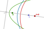
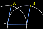
The Field of the Points on a Line
Let's continue with our construction process of the structure. Now we will
define the four elementary operations.
-
Addition: To obtain A + B, we reflect O in MAB obtaining a new
point on r.
-
Subtraction: To obtain A − B, we add A + B'.
-
Multiplication: We create the product by constructing similar
triangles, obtaining a new point on r.
-
Division: To obtain A/B, we multiply A x B–1. Division is not
commutative.
-
Order. The symmetry I' O I allows us to define a
ORDER RELATION:
A ≤ O :⇔AI' ≤ AI A ≤ B :⇔A − B ≤ O
Structure. Based on everything aforementioned, the set of points on
the line r, endowed with the operations of addition and multiplication as
defined,
constitutes a similar structure ("ordered field") to that of ℝ
(real numbers).
In fact, we can establish a bijection (isomorphism)
between both structures:
(r, O, +, ×) → (ℝ, +, ×)
correspond each point P on r to the real number –OP
if P<O and the real number OP if P≥O.
Note: Let us mark that we do not delve into the more
intricate question of how to geometrically construct all the points on the
line (completeness of the real line). We assume that every point
corresponds to a number and vice versa. However, if we wish to restrict
ourselves to points constructible with the mentioned operations, we can establish an isomorphism of those points (no
longer spanning the entire line) with the field of the constructible numbers.
|
The points on
a line are not the only geometric objects we can endow with the
structure of a field. We can apply the same concept to any other set of
objects that share the same definition, in which there is only one free
point residing on a line. Here are a few examples: |
|
Furthermore... |
The Field of Equidistant Perpendicular Bisectors
from a Fixed Point and another Free Point on a Fixed Line
Let r be the line passing through the fixed
points O and I. Let A be a point on r. We will call mA the perpendicular
bisector of the
segment OA.
Now, it's sufficient to extend all the operations
already seen between two points A and B to the corresponding ones between
perpendicular bisectors mA and mB.
If we align the coordinate origin with O
and point (1,0) with I, the point P corresponds to (p,0), allowing us to
represent the perpendicular bisector mP with the equation: x = p/2.
The Field of Equidistant Parabolas from a Fixed
Line and a Free Point on a Perpendicular Line
Let r be the line passing through the fixed
points O and I. Let d be the line perpendicular to r at point O, and
let A be a point on the line r. We will call dA the parabola of focus A
and directrix d.
Now, it's sufficient to extend all the operations
already seen between two points A and B to the corresponding ones between
the parabolas dA and dB.
If we align the coordinate origin with O
and point (1,0) with I, the point P will correspond to (p,0), allowing us
to represent the parabola dP with the equation: y²
= 2p x − p².
The Field of Equidistant Conics from a Fixed
Circle and a Free Point on a Diametral Line
Consider a circle with radius s centered at O, and let
A be a point on the line r passing through O and I. We will call sA the
conic of semiaxis s and foci O (fixed) and A.
Now, it's sufficient to extend all the operations
already seen between two points A and B to the corresponding ones between
the conics sA and sB.
If we align the coordinate origin with O
and point (1,0) with I, the point P will correspond to (p,0), allowing us
to represent the conic sP with the corresponding equation: (2x-p)²/s²
− 4y²/(p²-s²) = 1.
|
VERSATILITY
List of
Polylines
Lists allow a large amount of information to be grouped into a single
object. In this example, humble polygonal lines, lacking the elegance
found in many curves, make up for it with the versatility that their
grouping in a single list provides.
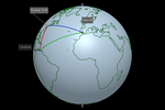
The Static Closed Polyline
We can import large amounts of data into a spreadsheet. In this
case, 6122 geographical coordinates from publicly available North American
Cartographic Information Society data
,
once cleaned up in a word processor and properly grouped, become lists.
Each point list is called by the Polyline command, so we finally
obtain
a list of polygonal chains whose arguments are point lists. Unlike
polygons, let's remember that the vertices of the polyline don't necessarily
have to lie in the same plane. Through this process, we achieve a
singular design: that of the Earth's coastlines. Thanks to this design, we
transform an ordinary sphere into a model of the Earth's surface.
Coast = {Polyline((5; 3.142; 1.204), (5; 3.117; 1.211), (5;
3.067; 1.22), (5; 3.031; 1.219), (5; 2.975; 1.223), (5; 2.967; 1.216), (5;
2.981; 1.204), (5; 2.96; 1.199), (5; 2.93; 1.214), (5; 2.896; 1.212), (5;
2.863; 1.216), (5; 2.832; 1.215), (5; 2.809; 1.212), (5; 2.787; 1.217), (5;
2.79; 1.23), (5; 2.775; 1.237), (5; 2.74; 1.24), (5; 2.67; 1.236), (5;
2.624; 1.25), (5; 2.609; 1.26), (5; 2.452; 1.271), (5; 2.429; 1.264), (5;
2.441; 1.248), (5; 2.413; 1.25), (5; 2.4; 1.245), (5; 2.366; 1.251), (5;
2.336; 1.246), (5; 2.308; 1.254), (5; 2.291; 1.236), (5; 2.264; 1.242), (5;
2.242; 1.256), (5; 2.252; 1.264), (5; 2.244; 1.275), ...
With this model [16] we can construct a scenario
in which we can engage in a multitude of activities. These activities
range from observing geographical elements (pole, meridian, parallel, cardinal point, equator,
tropic, polar circle, time zone...), to conducting analysis and
measurements (octant, latitude, longitude, course, rhumb line,
orthodromic distances, spherical triangle...).
Note: This model can serve as an excellent example
of the collaborative spirit that characterizes the resources created by
the GeoGebra community since its inception. Using it as a template, Chris
Cambré published books on GeoGebra about map projections
in Dutch and English, as well as another one about Mercator
.
Afterwards, Carmen Mathias translated both into Portuguese (,
).
Closing the circle, I translated them into Spanishl (,
).
This collaborative behavior reaches its peak in the GeoGebra forum
.
 If
we now add the apparent solar orbit, we'll have an armillary sphere
(or spherical astrolabe) that enables us to analyze the passage of time
(years, days, hours, GMT, UTC, seasons, zenith, obliquity of the ecliptic,
vernal point, equinox, solstice, celestial coordinates, analemma, celestial
horizon, sunrise, sunset, the 88 constellations, the zodiac,
the brightest stars...) [20]. If
we now add the apparent solar orbit, we'll have an armillary sphere
(or spherical astrolabe) that enables us to analyze the passage of time
(years, days, hours, GMT, UTC, seasons, zenith, obliquity of the ecliptic,
vernal point, equinox, solstice, celestial coordinates, analemma, celestial
horizon, sunrise, sunset, the 88 constellations, the zodiac,
the brightest stars...) [20].
Note: The Right Ascension
and Declination data for each star have been collected from
here.
The Self-Generated Static Polyline
At times, we can spare ourselves the task of importing vertices. The
iteration of a script associated with an animated slider (we will
delve into this procedure later) makes it easy to construct situations in
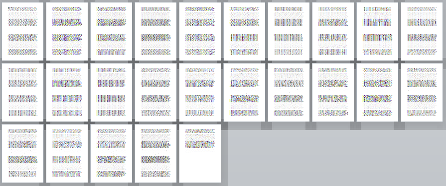
which the list of vertices for a polyline gradually expands on its own. A
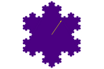
typical example of applying this method is the generation of fractals,
like the one illustrating the iterative process for creating the
well-known Koch snowflake and its corresponding anti-snowflake [29].
FLEXIBILITY: Elastic
Geometry
Elastic Geometry
Normally, a point either is or isn't in a specific position.
However, through scripts and vectors, we can introduce flexibility,
granting points the ability to move freely while attempting to maintain a
certain relationship with other points.
|
Instead of
fixing a specific position for each point, we will establish a
relationship with the rest of the points. |
Scripts
and Vectors
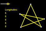
Our goal is to achieve an equilateral polygon with all its vertices
free. How can we close the polyline while keeping its vertices free (like
a carpenter's ruler)?
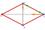
Or, starting from a polygon: How can we construct a rhombus while keeping the
fourth vertex free?
The solution lies in using scripts. For instance, a free point Q will
always remain 5 units away from the free point P if this script is
executed upon updating the position of P:
SetValue(Q, P + 5
UnitVector(Q−P))
and updating the position of Q executes the script:
SetValue(P, Q + 5
UnitVector(P−Q))
This way, in a rhombus, we can maintain the distance between vertices A and B
while both points remain free.
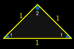
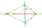
We can also represent types of triangles (right-angled,
isosceles, equilateral...) that retain their characteristics while
any of their three vertices can be moved.
This method also applies to preserving angles rather than distances.
Simply
modify the vector applied to the point, using the appropriate
rotation to readjust the angle. As an example, we can observe an equiangular
pentagon with all its vertices free.
Here, a result is included (published in 2015) that serves as a beautiful
example of the close relationship between geometry and algebra: "a polygon with n sides
is equiangular if and only if e2𝜋i/n is a complex root
of the polynomial of degree n–1 whose coefficients are the lengths of the
consecutive sides of the polygon"
.
Linkages
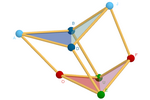
An example in space. This construction is based on the aforementioned principle
to maintain the distance (not the angles) between the vertices of a cube.
This way, an articulated cube is obtained, where its faces are not necessarily
flat, but consist of hinges formed by two isosceles triangles. The possible positions of its
vertices become difficult to analyze without resorting to this method
[4, 5, 32].
Animated Slider Scripts
However, we cannot generalize this method to polygons
with more than 4 sides, as adjusting the length of the fifth
side can disrupt the already adjusted ones. We would need iterative, continuous
readjustment, until achieving the desired result. Well, we can achieve
this continuous readjustment by utilizing a script that is executed
continuously, associated with the update of the value of an animated
slider.
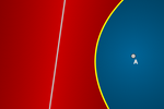
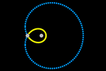
For instance, in the first scene, it might seem that P is a point on the
circle (with a radius of 4 centered at A), but in reality, it is a free point. By dragging it, it will return
to the circle because the script of the animated slider is executed
continuously. This script is:
SetValue(P, P + u)
where:
u = A - P + 4 UnitVector(P
− A)
We can add a coefficient (k) to control the speed: SetValue(P, P + k u)
If we add another vector, P will move towards the nearest intersection,
even if there is no intersection!
By doing the same with 5 points and 5 vectors, voilà! We can now maintain equidistance
among more than four points.
Fluid

By masking the polygon or the polyline with curves, for example using splines
,
we smooth the perception of the effect of the sum of internal forces
(which preserve the distance of the points) with external forces (which
apply a movement to the ensemble).
Amorphous
The achieved versatility is significant. For instance, we can literally make
figures "jump through the hoop". Let's remember that at no point
is the shape of the whole set determined; rather, it's a result of the
vectorial addition corresponding to the position reached at each moment.
Funicular Polygon
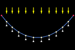
In this example, we start with a thread without appreciable mass from
which weights hang (the vertices of the polyline). The script of
slider-associated animation causes these vertices to vertically move downwards,
simulating gravity (external force), while the cohesive forces between
neighboring vertices (internal forces of the thread) limit this movement.
As we can observe, after a few seconds, the polyline takes on the shape of the
resulting funicular polygon
.
The vertices align themselves quite well with an ellipse. If we add more vertices, the
alignment
will come closer and closer to the theoretical parabola (infinite point
loads uniformly distributed horizontally). The catenary is not far off
either (it would be the result of removing the weight from the vertices
and adding uniform weight to the polyline thread: the loads are uniformly
distributed but not horizontally, rather along the curve, that is,
separated by the same arc length instead of the same horizontal length).
Newton's Principia
If there's a mathematical branch where traditional algebra and geometry
naturally blend, it's in analytic geometry, the core of dynamic
geometry programs like GeoGebra.
One of the key concepts in analytic geometry is that of a vector.
Its graphical representation as an arrow prompts us to think about
movement, about dynamism. We will use vectors to create dynamic
procedures, which are very simple yet incredibly powerful, allowing us to
address various situations.
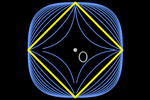
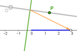
Vector Sum
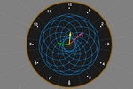
The hands of an analog clock can serve as an illustration of vectors. The
tip
of the hour hand traces a circle, much like the tip of the minute hand.
When we combine both vectors, we obtain a more intriguing path (this path
intersects itself at 11 points, assuming the minute hand is longer than
the hour hand, in 11 different directions, which means that within 12
hours, the vector sum of both hands coincides 121 times). If we also
include the second hand, vector addition leads to an even more complex
trajectory.
Vector sum open the door to the simulation of balances of forces. Thanks
to vectors, we can simulate forces, whether attractive or repulsive, that
compel a point to seek a relatively stable position (or path), one that is
in equilibrium with respect to other forces or constraints.
Circular Confinement Between Repelling Points
We can imagine the points as charged particles that repel each other and
are confined to the same circle. Each point is associated with the sum of
the repulsion vectors from the other points. In this way, the points
automatically readjust themselves, seeking the equilibrium position. As
expected, this position always corresponds to the vertices of a regular
polygon inscribed in the circle.
Square Confinement Between Repelling Points
If we replace the circle with a less symmetrical shape, such as a square,
regular distributions are no longer possible in all cases. Nevertheless,
the equilibrium position is still always reached at the perimeter
boundary.
Spherical Confinement Between Repelling Points
If we transition from the circle to the sphere (the Thomson problem
,
a particular case of one of the eighteen unsolved mathematical problems
proposed by mathematician Steve Smale
in the year 2000), perfect regularity is no longer achievable since there
are no Platonic solids with 5 or 7 vertices, for example.
Moreover, it is not even true that equilibrium is always reached in
perfect regularity! In fact, with 8 vertices, the cube is not the
configuration that achieves equilibrium. Note also that in most cases,
polyhedra with triangular faces appear (but generally not equilateral,
hence they are not deltahedra
).
Minimal Path
The vectors governing the movements of particles can be undefined. At each
step, we can try various vectors and choose the one that best suits our
objective.
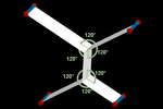
In this example, a simulation of the well-known soap film experiment, the
particles try various movements before settling on those that minimize the
total length of the profile and, therefore, the total area of the surface
(in this case, they head towards the Steiner points [23]
of the four vertices). The angles of the sheets are 120º due to the
uniformity in the direction of the Euclidean distance.
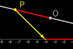
Orbit
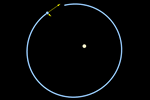
Let's take a closer look at how simple it is, thanks to the continuously
animated slider, to observe the elliptical motion of the Earth around the
Sun without the need for infinitesimal analysis
[20].
Note: This construction was made based on the
suggestion of my colleague Julio Valbuena, who adapted the idea presented
by Richard Feynman in his famous book The Feynman Lectures on
Physics (volume I, 9-7, Planetary motions), see
Bibliography.
We place the point S (Sun) at the coordinate center and a point T (Earth)
with initial velocity vector v. If d is the distance TS and k is a
positive constant, we have the gravitational force vector:
g = k/d² UnitVector(S–E)
Now we just need to introduce an auxiliary slider so that, whenever it is
updated, it executes the very simple script:
SetValue(v, v + 0.03 g)
SetValue(E, E + 0.03 v)
And we already have elliptical motion! (Note that we haven't used any
equations or geometric loci.)
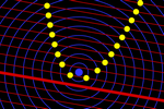
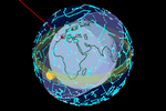
Chaos
The previous construction explains the nearly perfect elliptical orbits of
planets around the Sun. The "almost" is determined by the presence of
other bodies. Fortunately for Earthlings, the orbits of the other planets
are sufficiently distant not to disrupt our solar year too much. Here, we
see what would happen if that weren't the case. This is a simplification
(two bodies orbiting another in the same plane) of the famous
"three body problem"
.
It is impressive to observe how such a simple construction can transform order
into chaos [24].
Bubbles (using JavaScript)

We can use vectors to modify the movement of an object based on its
distance from another object, allowing, for example, collision detection.
The problem is that if there are many objects (n), the number of events
will be high, as it grows with the square of the number of objects: n(n–1)/2.
In these cases, it's best to replace the GeoGebra scripts with faster
JavaScript code, as demonstrated in this construction. It shows elastic
collisions, and you can verify thee conservation of total kinetic
energy at all times.
Tensegrities
Elastic geometry allows us to find equilibrium situations between
different forces. An interesting application is tensegrity structures,
composed of bars and tensioned cables that hold them together.
Tensegrity
When we connect different vertices, we obtain the graph of a network [25].
But if the connections are made up of bars and springs, we can achieve
that in certain positions, the tension of the springs balances out in a
stable structure, called a tensegrity
.
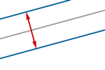
Here is an example in the plane. Because the rhombus is a parallelogram,
the forces at each vertex cancel out, so the structure remains in stable
equilibrium in any position, as long as the horizontal and vertical
tensions are equal.
|
Furthermore... |
Calculation of Tensions
If we start with an arbitrary quadrilateral,
tensegrity is only achieved for certain positions and tensions. If we vary
any of those positions or tensions, the structure will automatically seek
the new equilibrium position.
The key is in the vertices: the vector sum of the forces involved must
always be zero.
|
Tensegrity of a Triangular Prism
(simplex)
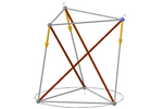
Let's move into three-dimensional space. One of the simplest tensegrities
starts with a right prism whose bases are equilateral triangles. We place
bars along its lateral edges and cables everywhere else. If we tension the
cables, tensegrity is achieved when one of the bases rotates exactly 150°
relative to the other.
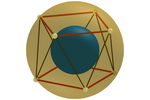
Icosahedral Tensegrity by Tensioning Cables
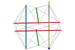
One of the pioneers of tensegrities, Buckminster Fuller, showed particular
interest
in this type of tensegrity. It consists of a structure formed by three
pairs of parallel bars, perpendicular to each other, tensioned by cables.
The whole structure constitutes a non-convex icosahedron, known as the Jessen's icosahedron
,
whose vertices do not occupy the same positions as in a regular
icosahedron.
We start with bars attached in pairs. When tensioned, the bars separate
until the direction of the resulting force aligns with that of the bar.
The ratio between the length of each bar and each cable will then be exactly
.png) (≈1.63).
Note that in a regular icosahedron, this ratio is the golden ratio
(≈1.62). We can observe that the angle of the faces of Jessen
Icosahedron is 90º. (≈1.63).
Note that in a regular icosahedron, this ratio is the golden ratio
(≈1.62). We can observe that the angle of the faces of Jessen
Icosahedron is 90º.
Icosahedral
Tensegrity by Extending Bars
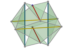
We can achieve the same result by operating in reverse. Instead of
tensioning the cables, we try to extend the six bars as much as
possible. In this case, we start with a cuboctahedron. We place the
bars and stretch them to their maximum length while maintaining the
original length of the edges (the cables) of the cuboctahedron.
Conclusions
It is true that the current GeoGebra is much more complex than its first version
from a couple of decades ago. We have so many procedures and commands that
advance planning is necessary to decide, depending on the context, which of them
we really need to achieve our educational objectives.
In this presentation, we have seen with numerous examples that GeoGebra allows
us to tackle a wide variety of problems with minimal means. While CAS commands
make it possible to transcend, in some cases, the difficulty of introducing
algebra in secondary education, lists, vectors, and scripts add ease in
representing flexible, dynamic, and interactive situations. And often, these
situations are tremendously attractive, both in terms of aesthetics and in the
sense that they invite us to explore our own constructions (let's remember the
Ikea effect), which promotes the acquisition of mathematical competence.
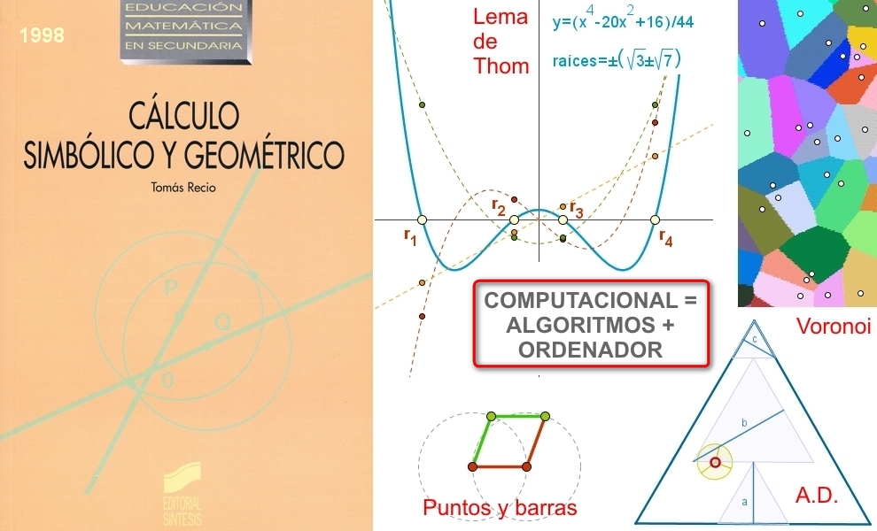
Acknowledgments
While in this presentation I did not intend to follow the
expositional lines set out by Tomás Recio in his 1998 book Cálculo Simbólico y Geométrico
[30], I must acknowledge the enormous
influence that this book, which I highly recommend, has had on my
understanding of both Mathematics and its teaching. Additionally, I
want to thank Tomás for his suggestions and clarifications on some
of the points discussed here.
References
[1] Álvarez, J.L. and Losada, R. (2011).
El proyecto
Gauss. SUMA Magazine,
No. 68, pp. 17-25.
[2] Arranz, J.M., Losada, R., Mora, J.A.
and Sada, M. (2008).
El cristo de la farola. Divulgamat, Royal Spanish Mathematical
Society. GeoGebra Book:
G⁴D en Divulgamat
[3] Arranz, J.M., Losada, R., Mora, J.A. and Sada, M. (2010).
De luz y de color. Divulgamat, Royal Spanish Mathematical
Society.
GeoGebra Book:
G⁴D en Divulgamat
[4] Arranz, J.M., Losada, R., Mora, J.A., Recio, T.
and Sada, M. (2009).
GeoGebra on the rocks. Dynamic Geometry Geometry Learn.
[5] Arranz, J.M., Losada, R., Mora, J.A., Recio,
T. and Sada, M. (2011).
Modeling the cube using GeoGebra. Model-Centered
Learning: Pathways to mathematical understanding using GeoGebra, pp.
119-131. Eds. L. Bu & R. Schoen (Eds.). Rotterdam: Sense Publishers.
[6] Calatayud, P. (2018).
El problema de la separación de elipses y elipsoides: una aplicación de la
eliminación de cuantificadores.
[7] Hohenwarter, M. (2006).
GeoGebra – didaktische Materialien und Anwendungen
für den Mathematikunterricht.
[8] Kovács, Z.
(2021).
Two almost-circles, and two real ones. Mathematics
in Computer Science 15, pp. 789–801.
[9] Losada, R. (2007).
La chica en
el espejo. GeoGebra Book.
[10] Losada, R. (2007).
GeoGebra: la eficiencia de la intución.
The Gazette of the Royal Spanish Mathematical Society, Vol. 10.1, pp. 223-239.
[11] Losada, R. (2009).
GeoGebra en
la Enseñanza de las Matemáticas. Ministry of Education. CD-ROM. ISBN: 978-84-369-4794-6.
[12] Losada, R., Recio, T. and Valcarce, J.L. (2009).
Sobre el descubrimiento
automático de diversas generalizaciones del Teorema de Steiner-Lehmus.
Puig Adam Society Newsletter, No. 82, pp.
53-76. Complutense University of Madrid. English version:
On the automatic discovery of Steiner-Lehmus generalizations.
[13] Losada, R. and Álvarez, J.L. (2010).
GeoGebra en
la Educación
Primaria. Ministry of Education. CD-ROM.
ISBN: 978-84-369-4909-4.
[14] Losada, R. and Álvarez, J.L. (2011).
Proyecto Gauss.
Institute of Educational Technologies,
Ministry of Education.
[15] Losada, R. (2011).
Dimensiones.
GeoGebra Book.
[16] Losada, R. (2011).
Modelos.
GeoGebra Book.
[17] Losada, R., Recio, T. and Valcarce, J.L. (2011).
Equal Bisectors at a Vertex of
a Triangle. Computational Science and Its Applications - ICCSA.
[18] Losada, R. and Recio, T. (2011).
Descubrimiento
automático en un problema centenario. The Gazette of the
Royal Spanish Mathematical Society, Vol. 14.4, pp. 693-702.
[19] Losada, R. (2014).
El
color dinámico de GeoGebra. The Gazette of the Royal Spanish
Mathematical Society. Vol. 17 (nº 3), 525–547. GeoGebra Book:
Color
dinámico.
[20] Losada, R. (2016).
La Tierra y
el Sol. GeoGebra Book. English version: Earth and
Sun.
[21] Losada, R. (2017).
La
percepción del tamaño. GeoGebra Book.
[22] Losada, R. (2018).
Animaciones
automáticas. GeoGebra Book.
[23] Losada, R. (2018).
Autómatas.
GeoGebra Book.
[24] Losada, R. (2018).
Billares:
orden y caos. GeoGebra Book
[25] Losada, R. and Mora, J.A. (2021).
Redes y grafos. Las comunicaciones y la logística.
Mathematics for a better world exhibition. Red DiMa, International
Mathematics Day. GeoGebra Book:
Redes y
Grafos.
[26] Losada, R. and Recio, T. (2021).
Mirando a los
cuadros a través de los ojos de Voronoi. Puig Adam Society
Newsletter, Vol. 112, pp. 32–53. Complutense University of Madrid. GeoGebra Book:
Voronoi
paintings.
[27] Losada, R. (2022).
Mapas de c@lor con GeoGebra. SUMA
Magazine, No. 102, pp. 43-57.
GeoGebra Book:
Mapas de c@lor
con GeoGebra.
[28] Losada, R. and Recio, T. (2023).
Inclinando la botella de Piaget con
GeoGebra Discovery. Puig Adam Society Newsletter, Vol. 115, pp.
43-86. Complutense University of Madrid. GeoGebra Book:
Inclinando
la botella de Piaget con GeoGebra Discovery.
[29] Pérez, A., Sada, M. and Losada, R. (2021).
Fractales, la Geometría del Caos. Mathematics for a better
world exhibition. Red DiMa, International Mathematics Day.
[30] Recio, T. (1998).
Cálculo Simbólico y Geométrico, Secondary
Mathematics Education collection, Editorial Síntesis, Madrid.
[31] Recio, T., Losada, R., Kovács, Z.
and Ueno, C. (2021).
Discovering
Geometric Inequalities: The Concourse of GeoGebra Discovery, Dynamic
Coloring and Maple Tools. Mathematics 9 (20), 2548.
[32] Recio, T., Losada, R., Tabera, L.F. and Ueno, C. (2022).
Visualizing a Cubic Linkage through the Use of CAS and DGS.
Mathematics 2022, 10(15),
2550; https://doi.org/10.3390/math10152550. GeoGebra Book:
Mecanismos.
English version:
Linkages.
Bibliography
-
Arranz, J.M., Losada, R., Mora, J.A. and Sada, M. (2008).
Arcos con geometría dinámica. Matematicalia,
Royal Spanish Mathematical Society, Vol. 4.1. GeoGebra Book:
Arte
y Geometría: Arcos
-
Arranz, J.M., Losada, R., Mora, J.A. and Sada, M. (2008).
Conjeturas a partir de los puntos medios. Divulgamat, Royal
Spanish Mathematical Society. GeoGebra Book:
G⁴D en Divulgamat
-
Arranz, J.M., Losada, R., Mora, J.A. and Sada, M. (2008).
La percepción tridimensional. Divulgamat, Royal Spanish
Mathematical Society. GeoGebra Book:
G⁴D en Divulgamat
-
Arranz, J.M., Losada, R., Mora, J.A. and Sada, M. (2008).
Geometría en rosetones góticos. Divulgamat, Royal
Spanish Mathematical Society. GeoGebra Book:
G⁴D en Divulgamat
-
Arranz, J.M., Losada, R., Mora, J.A. and Sada, M. (2009).
Mosaicos con GeoGebra. Lemniscata
collection, No. 7, pp. 57-87. Editorial
Anaya. GeoGebra Book:
Arte y Geometría: Mosaicos
-
Arranz, J.M., Losada, R., Mora, J.A. and Sada, M. (2009).
Realities from GeoGebra. MSOR Connections Vol. 9 No. 2.
Spanish version:
Realidades de GeoGebra SUMA Magazine. No. 67, pp. 7-20.
Reissued on the occasion of
No. 100 in 2022. GeoGebra Book:
Realidades
de GeoGebra.
-
Botana, F., Kovács, Z., Recio, T. and Vélez, M.P. (2020).
Hacia
un autómata geómetra. The Gazette of the Royal
Spanish Mathematical Society, Vol. 23.2, pp. 343–371
-
Burkhardt, R.W. (2008).
A Practical Guide to Tensegrity Design.
-
Carrillo, A. and Recio, T. (2020).
De Curva a Curva,
con GeoGebra. Puig Adam Society Newsletter, No. 110.
-
Durán, A.J., Mora, J.A., Pereiro, D., Losada, R., Muñoz, J.L., Arranz, J.M.
(2021).
Matemáticas y belleza. Mathematics for a better world
exhibition. Red DiMa, International Mathematics Day.
-
Feynman, R., Leighton, R.B. and Sands, M. (1963).
The Feynman Lectures on Physics, Mainly Mechanics, Radiations and Heat,
Volume I. Addison-Wesley.
-
Goicolea, J.M. (2021).
Cálculo de Cables. Polytechnic University of Madrid.
-
de Guzmán, M. (2002).
Tensegridad. De la escultura a la célula. Ars Medica.
Humanities Magazine.
-
Losada, R. (2002).
All Lights y Lights Out: una investigación entre luces y sombras.
SUMA Magazine. No. 40, pp. 25-41. GeoGebra Book:
Juegos de
iluminación (con soluciones). English version:
Lights Out (games with solutions).
-
Losada, R. (2010).
Isometrías.
GeoGebra Book.
-
Losada, R. (2010).
Estadística
y Probabilidad. GeoGebra Book.
-
Losada, R. (2011).
Aritmética y
cálculo mental. GeoGebra Book.
-
Losada, R. (2011).
Ecuaciones y
sistemas. GeoGebra Book.
-
Losada, R. (2011).
Funciones.
GeoGebra Book.
-
Losada, R. (2011).
Música y
matemáticas. Divulgamat, Royal Spanish Mathematical
Society. GeoGebra Book:
Música y
Matemáticas
-
Losada, R. and Álvarez, J.L. (2011).
Los applets de funciones en el Proyecto Gauss. UNO
Magazine,
No. 58, pp. 25-37. Editorial Graó.
-
Losada, R. and Álvarez, J.L. (2012).
Estadística y probabilidad en el Proyecto Gauss.
UNO Magazine,
No. 59, pp. 26-39. Editorial Graó.
-
Losada, R. and Álvarez, J.L. (2012).
La hoja de cálculo de GeoGebra.
UNO Magazine, No. 61, pp.
55-66. Editorial Graó.
-
Losada, R.
(2016).
Geogebra en el aula, un descubrimiento gradual.
UNO Magazine, No. 71, pp. 13-19. Editorial Graó.
-
Losada, R. (2021).
Cambio de
sistema de referencia. GeoGebra Book.
-
Losada, R. (2021).
Variable
compleja. GeoGebra Book.
-
Losada, R. (2021).
Julia y
Mandelbrot. GeoGebra Book.
-
Petrovic, M., Malesevic, B., Banjac, B. and Obradovic, R. (2014).
Geometry of some
taxicab curves.
-
Plaza, S. and Gutiérrez, J.M. (2013).
Dinámica del método de Newton.
University of La Rioja.
-
Ramellini, G.,
Losada, R. and Muñoz, J. (2021).
Juegos y Matemáticas. Mathematics for a better world
exhibition. Red DiMa, International Mathematics Day.
GeoGebra Books:
Juegos,
Rompecabezas,
Matemágicas.
-
San Segundo, F. (2010).
Effective
algorithms for the study of the degree of algebraic varieties in
offsetting processes.
|